Read my previous post to learn about some high level concepts of machine learning.
In this blog, we will use these to build features, train a model and then use it to infer predicted points for each player for their next fixture.
The code for this blog can be found here and here.
You can go back to the case study here.
Features
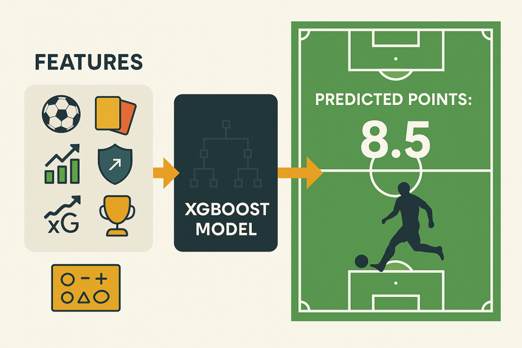
To train a model, we start with a dataset packed with features that influence the target variable. For us, that target is the total FPL points a player scores in a fixture. The more useful data we feed in, the better the model can infer player or team strength.
We don’t care about names or clubs. Whether it’s Haaland or Antony, Arsenal or Wolves, the identity doesn’t matter. What matters is recent performance – because form is often the best predictor of what happens next.
This may mean that we often predict an unknown player to be top scorer next week because they miraculously scored a hattrick last week, but that’s FPL, right?
From the FPL API, we pull stats like:
- Minutes played
- Goals and assists
- Expected goals (xG) and Assists (xA)
- Clean sheets and goals conceded
- Cards and defensive actions
These exist in our silver layer at a per-player, per-fixture level. We roll them up to team-level stats too (e.g., team xG).
To capture form, we use a 5-gameweek window. For each stat, we create:
- Rolling totals (sum over the last 5 gameweeks)
- Averages (rolling total / games played – fewer than 5 early on)
Putting this together, we now have a dataset with:
- player_key and fixture_key to model and debug later
- Rolling and Average player-level stats over the previous 5 gameweeks
- Rolling and Average team-level stats for the player’s team over the previous 5 gameweeks
- Rolling and Average team-level stats for the opponent team over the previous 5 gameweeks
- Actual FPL Points gained by the player in that fixture
Note: Our dataset goes back to 2016/17, before stats like xG and xA existed. When a feature isn’t available, we set its value to -1. This is because 0 has meaning (e.g. zero goals), and we don’t want the model to confuse “missing” with “actual zero”. This approach also applies to newer stats, like defensive contributions introduced in 2025/26.
Training and Measuring Models
We split the dataset into an 80/20 train-test split using player gameweek data from 2021/22 onwards. This cut-off reflects changes in post-COVID football and the increased availability of advanced stats like xG and xA.
We then tested several scikit-learn models: RandomForest, GradientBoosting, Ridge, Lasso, SVR, and XGBoost.
To measure performance, we used two metrics:
- R² (Coefficient of Determination): Shows how much of the variance in the target variable the model explains. An R² of 1 means perfect prediction; 0 means the model explains nothing.
- RMSE (Root Mean Squared Error): Measures the average prediction error in the same units as the target. Lower is better because it means predictions are closer to actual values.
XGBoost outperformed the others, so we narrowed down to that and ran hyperparameter tuning using GridSearch. We adjusted:
- n_estimators
- max_depth
- learning_rate
- subsample
- colsample_bytree
After optimisation, we saved the best model for inference.
For context, most fantasy football predictive models have an R² between 0.3 and 0.5, due to the randomness in football and fantasy performance.
Our model achieved R² = 0.466 and RMSE = 1.721.
An R² of 0.466 means the model explains nearly half the variance in player points, which is strong for a domain as unpredictable as football.
The RMSE of 1.721 means predictions are usually within about 1.7 points of the actual score, which is very usable for decision-making in FPL. However, FPL is quite a low-scoring game with players of the week only scoring 15-20 points, so 1.7 could be fairly high.
Overall, I am happy with this for the first run-through for an MVP!
Retraining and Inference
Our pipeline runs every gameweek, so the latest trained model won’t include the most recent fixture data. Before making predictions, we retrain the model with the new gameweek points. If the updated model performs better than the current version (based on R² and RMSE), we save it as the new production model.
For inference, we start by pulling all players and their upcoming fixtures. Then we build the same features used during training:
- Player form over the last 5 gameweeks
- Team form
- Opponent team form
The only missing piece is the target variable, total_points, which we now predict. Using the most recent version of the trained model, we generate predicted points for each player in the next fixture and write these predictions back to our feature layer tables.
Now we have the silver and feature layers, which contain all the necessary data to build the gold layer!
BW

